
Space Reporting
Space Reporting
Let's look at rocketry
We have rich datasources from government and hobby sources, which makes space datasets interesting to work with.
And a lot of people like space, so that's a bonus.
Today we'll work with data from this fantastic source:
Info
McDowell, Jonathan C., 2020. General Catalog of Artificial Space Objects, Release 1.8.0 , https://planet4589.org/space/gcat
What are we going to do?
Let's make two views; one view of where things go up (rockets), and one where things go around (satellites).
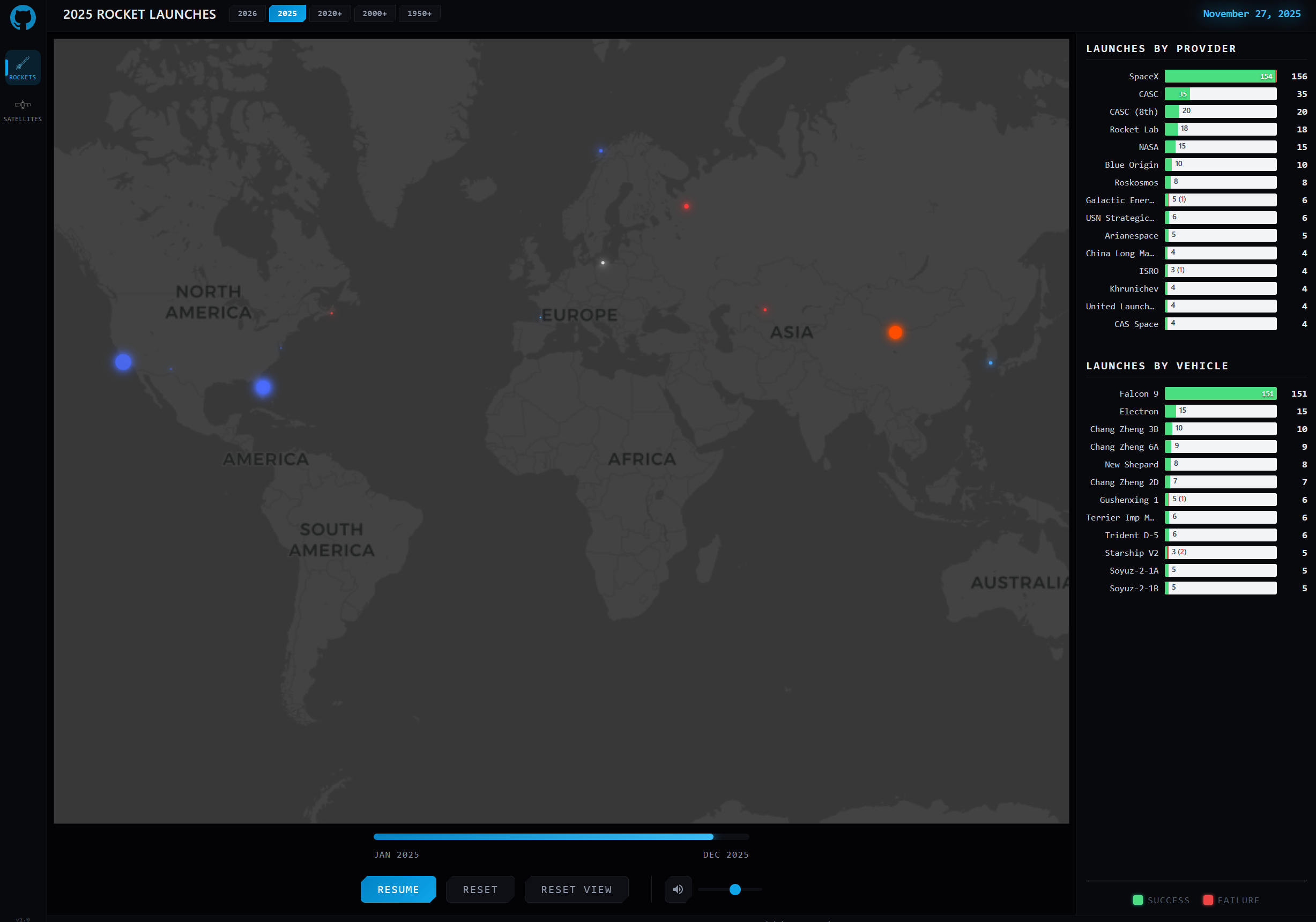
Our "where things go up view" is going to look like this, for example:
Links
If you just want to skip ahead to the final product, links are here:
Tips
Load with sound on if you can!
By the Numbers
Before we get into the details, let's take a tour of highlights.
Tips
Every chart below is generated directly from the public gcat_space model with the Trilogy CLI - each one is a copy into png ... from chart ... statement against the same parquet files the dashboards read.
The catalog goes back to Sputnik in 1957, so the whole space age fits on one axis.
Things that go up
The launch cadence
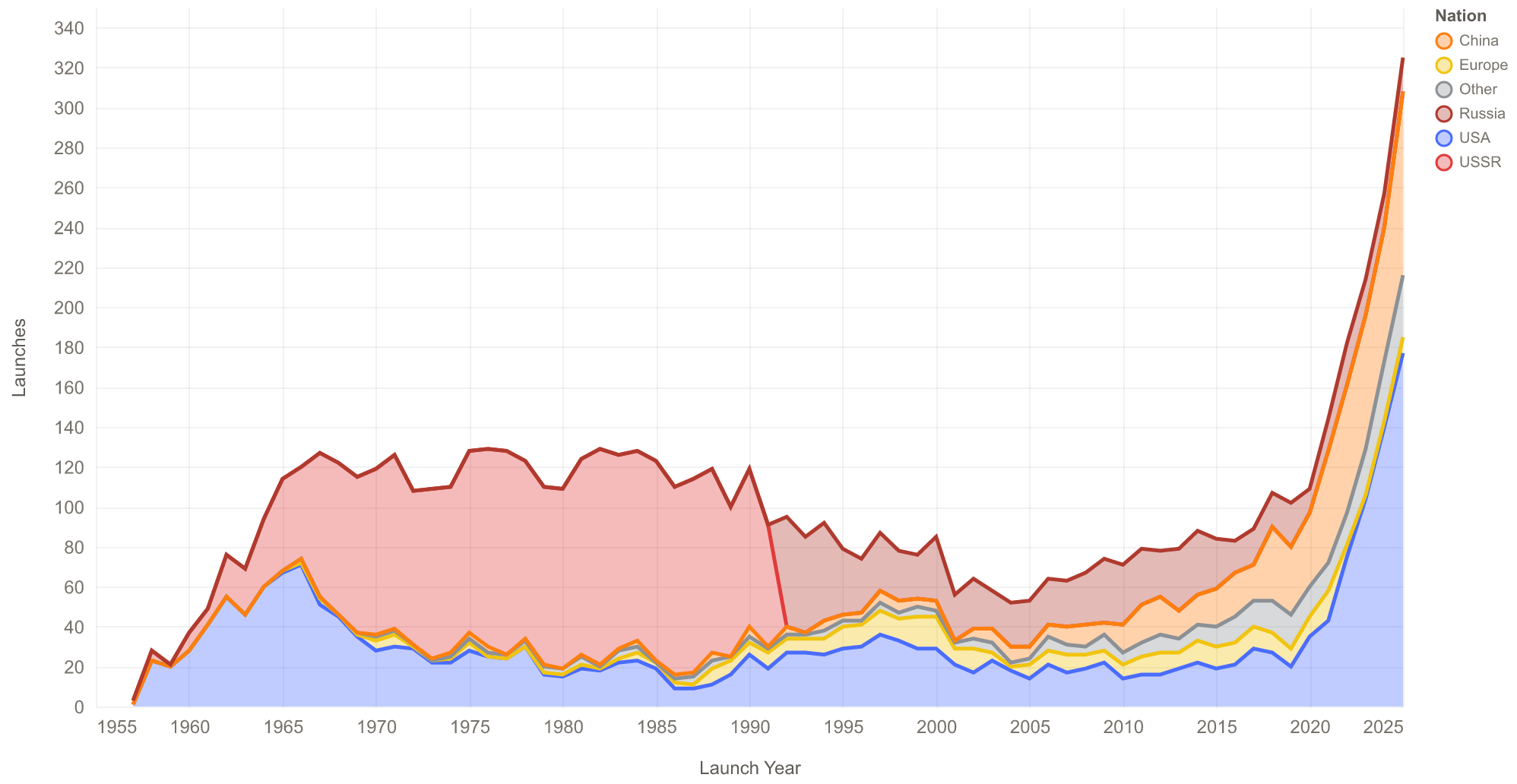
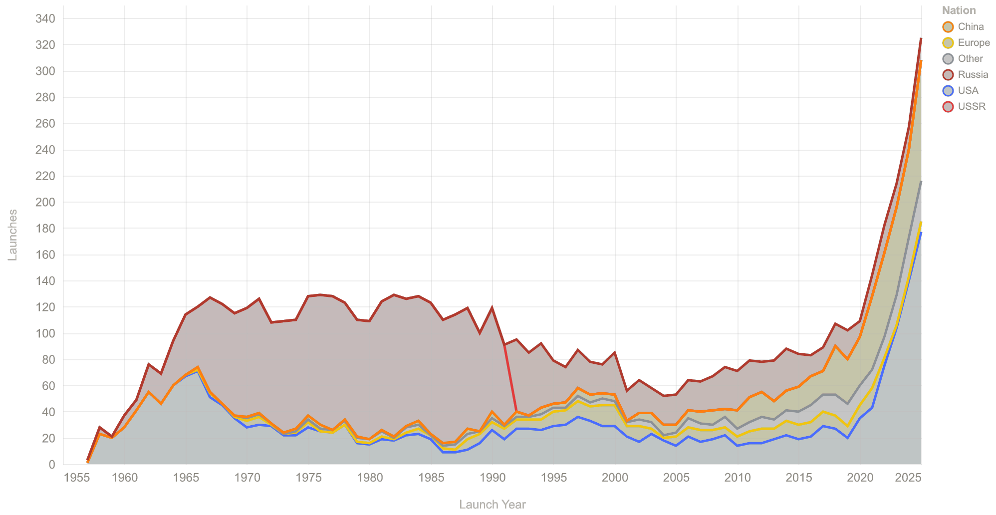
Orbital launches per year, stacked by who did the launching, is a story of geopolitics. The USSR (red) and the USA (blue) face off throughout the Cold War, but the USSR drops off as the wall falls, transforming to Russia (the darker red carrying the same program forward). The USA (blue) holds steady while he post-Soviet lull bottoms out around ~55 launches in the mid-2000s, and then the modern surge arrives on two engines: a reusable-rocket boom in the USA and a rising China (orange), pushing the total to 325 in 2025, an all-time high.
(The country colors here aren't the chart library's defaults - the query emits a ::hex column next to each nation and Trilogy maps each series to that literal color, so USSR/Russia read as red and the USA as blue on purpose.)
Launch Cadence Query
import launch;
import std.color; # the 'hex' type; a ::hex column drives the series colors

where
    launch_type_code = 'O'
    and launch_date.year >= 1957
    and launch_date.year <= 2025
    and state.short_e_name is not null
    and state.short_e_name != '-'
select
    launch_date.year as launch_year,
    CASE
        WHEN state.short_e_name = 'USA' THEN 'USA'
        WHEN state.short_e_name = 'USSR' THEN 'USSR'
        WHEN state.short_e_name = 'Russia' THEN 'Russia'
        WHEN state.short_e_name = 'China' THEN 'China'
        WHEN state.short_e_name IN ('France','ESA','ELDO','Italy','UK','Germany') THEN 'Europe'
        ELSE 'Other'
    END as nation,
    CASE
        WHEN state.short_e_name = 'USA' THEN '#4A6CFF'
        WHEN state.short_e_name = 'USSR' THEN '#E23B3B'
        WHEN state.short_e_name = 'Russia' THEN '#B03A2E'
        WHEN state.short_e_name = 'China' THEN '#FF7F0E'
        WHEN state.short_e_name IN ('France','ESA','ELDO','Italy','UK','Germany') THEN '#F1C40F'
        ELSE '#8C9196'
    END::hex as nation_color,
    count(id) as launches
order by
    launch_year asc;
Who's doing the launching?
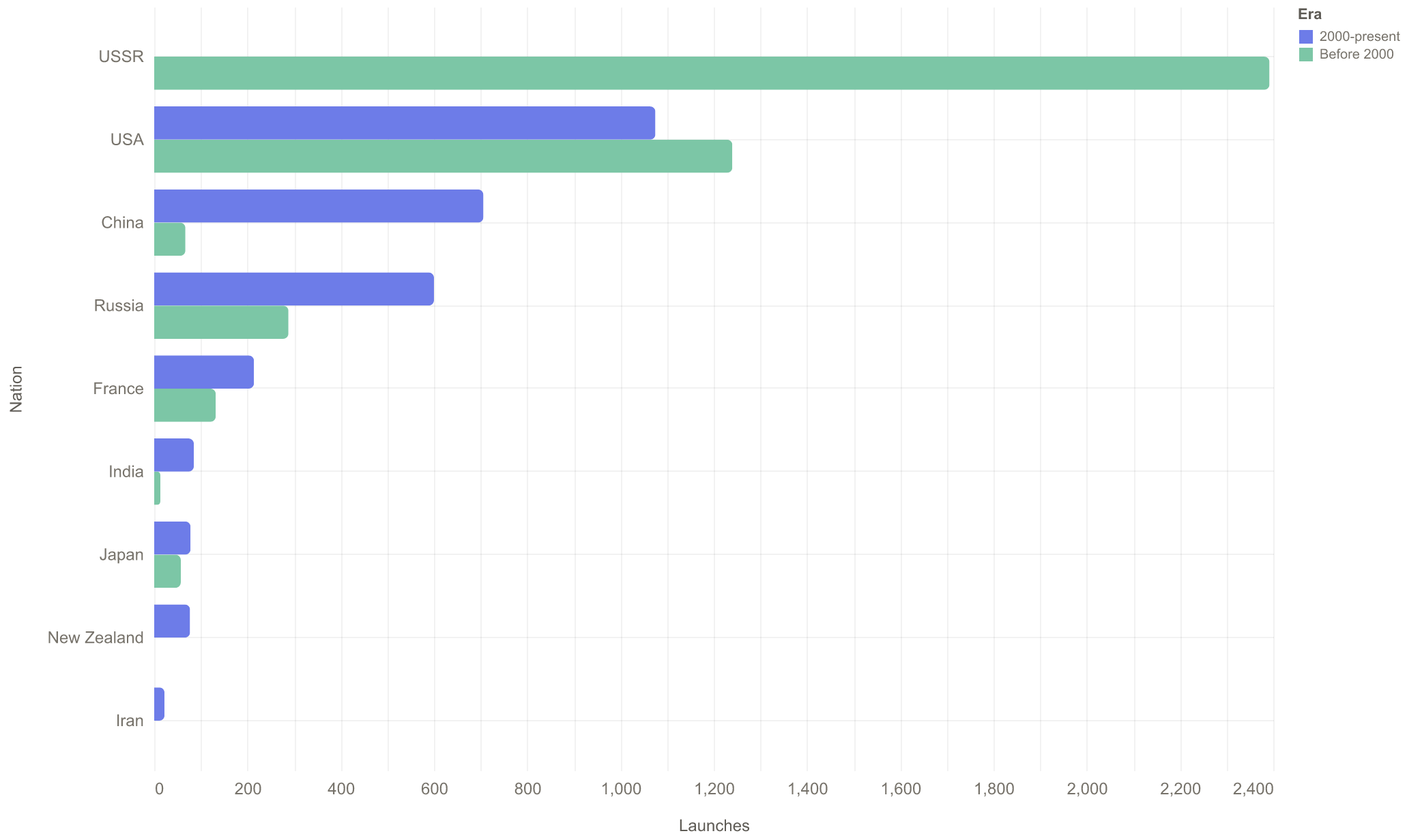
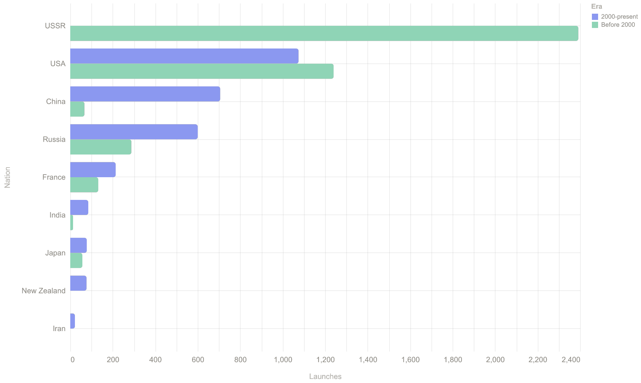
Split each nation's launches into before-2000 and 2000-present and the modern day space-race emerges. The 20th century was basically two players: the USSR and the USA, with a handful of others (France, Japan) barely registering.
The 21st century is a different map. China went from a rounding error (67 launches) to over 700, nearly all of it post-2000. Russia carries the Soviet program forward. And a whole tier of newer entrants is almost entirely modern: India's starts to put on a show alongside a longer tail - including Iran, and New Zealand (RocketLab) as well as the Japan/European and other small-tier launchers.
Launch Nations Query
import launch;

where
    launch_type_code = 'O'
    and state.short_e_name IN (
        'USA','USSR','Russia','China','France','Japan','India','New Zealand','Iran'
    )
select
    state.short_e_name as nation,
    case when launch_date.year < 2000 then 'Before 2000' else '2000-present' end as era,
    count(id) as launches
order by
    launches desc;
The workhorses
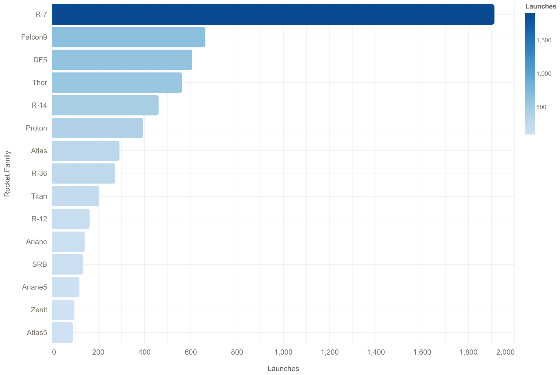
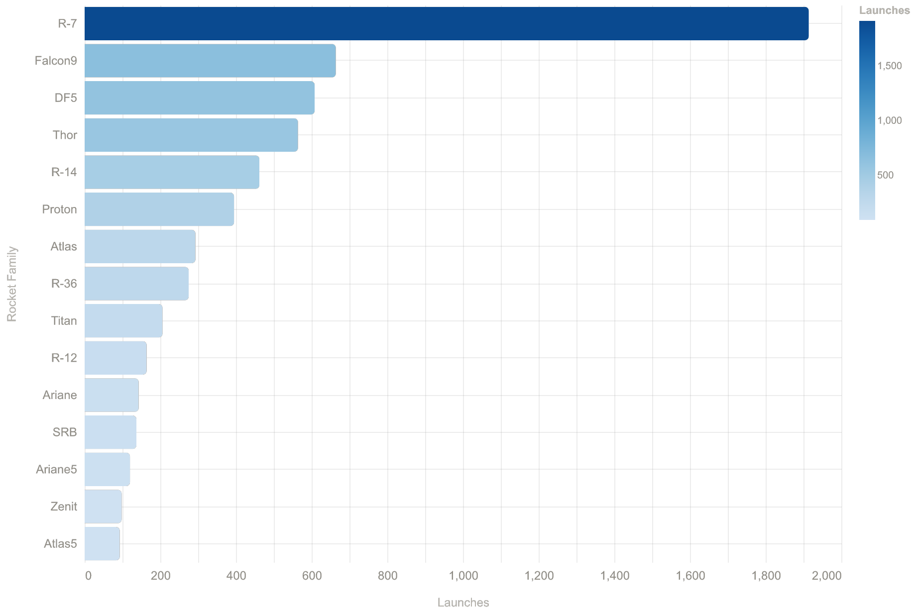
Group launches by vehicle family and we still have one undisputed champion the Soviet R-7, first flown in 1957 and still flying today as Soyuz, with close to 2,000 orbital launches. Starship is coming - but will it be in time to keep SpaceX's Falcon 9 from dethroning the old stalwart?
Note that some entries here (R-14, R-36, DF5) started life as missiles - the catalog counts every orbital attempt, not just civilian ones.
Top Vehicles Query
import launch;

where
    launch_type_code = 'O'
    and vehicle.family is not null
    and vehicle.family != '-'
select
    vehicle.family as rocket_family,
    count(id) as launches
order by
    launches desc
limit 15;
Getting good at it
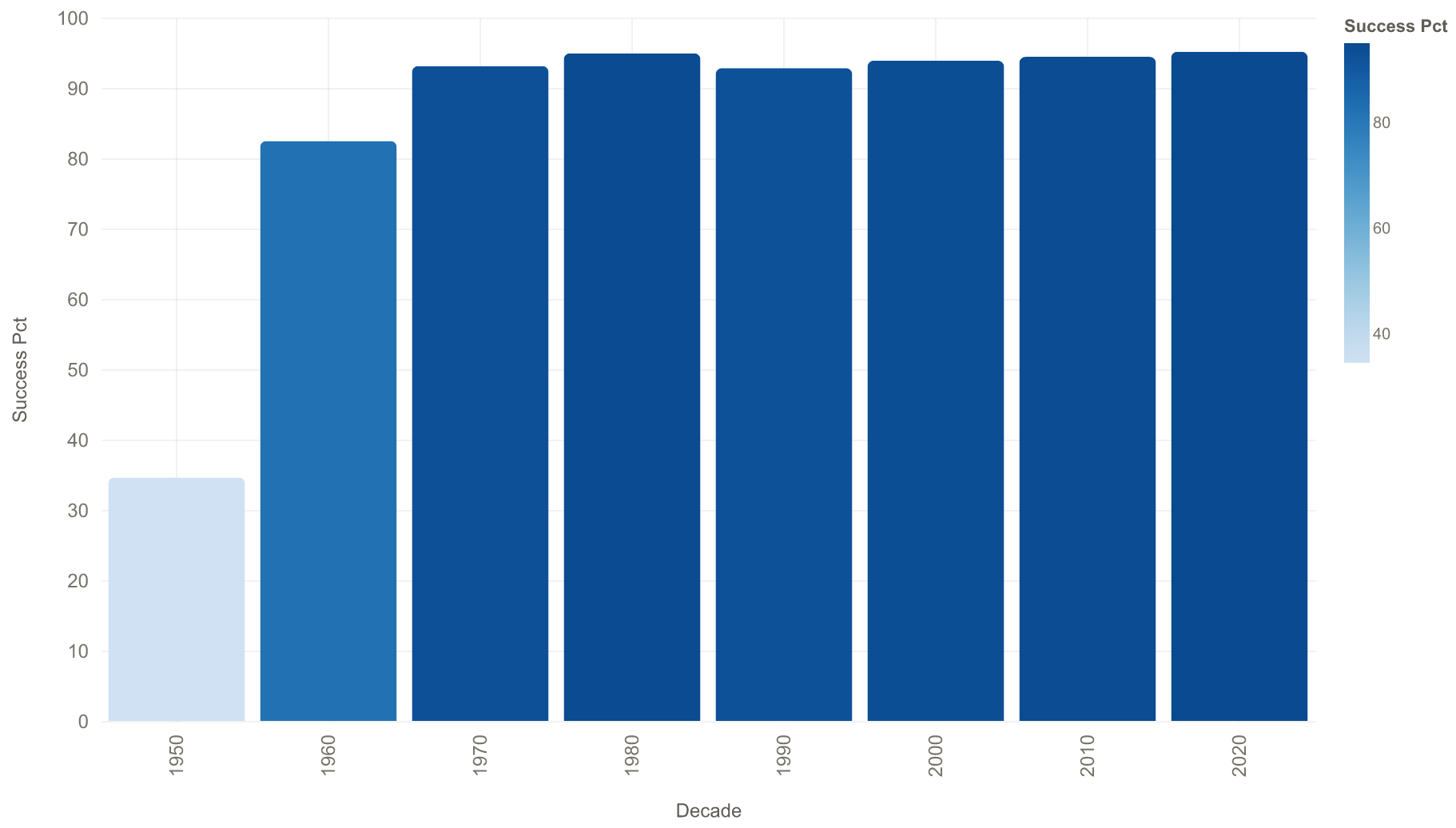
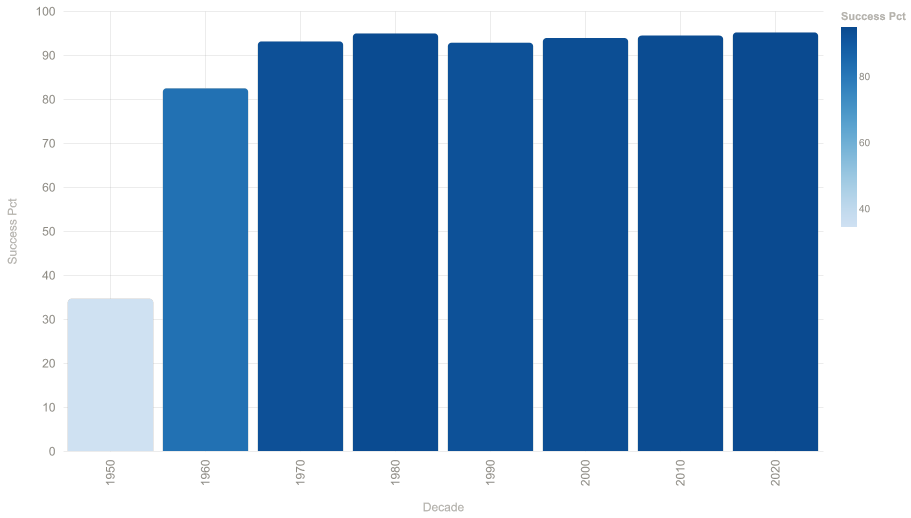
Rocketry and fireworks used to be closer cousins. In the 1950s barely a third of orbital attempts fully succeeded; by the 1960s that was 82%, and from the 1970s onward it settles into a plateau north of 93%. That's still an A-, though - Rocket Science is a watchword for difficulty for a reason.
Eyes will be on 2030+ to see if it can approach the reliability of airlines.
Success Rate Query
import launch;

where
    launch_type_code = 'O'
    and success_flag is not null
    and launch_date.year >= 1950
select
    (launch_date.year - launch_date.year % 10) as decade,
    avg(case when was_complete_success then 100.0 else 0.0 end) as success_pct
order by
    decade asc;
Things that go around
The shape of low Earth orbit
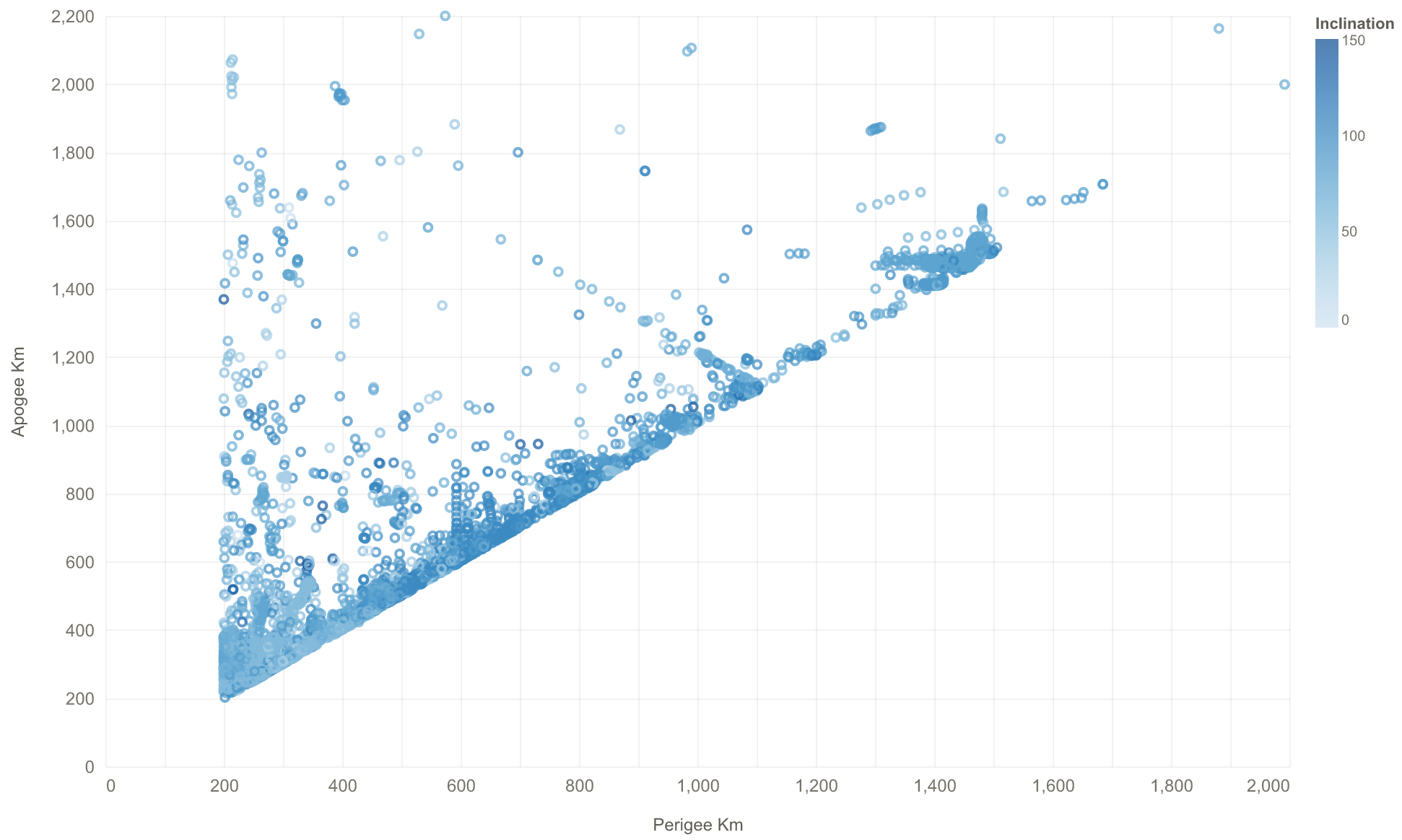
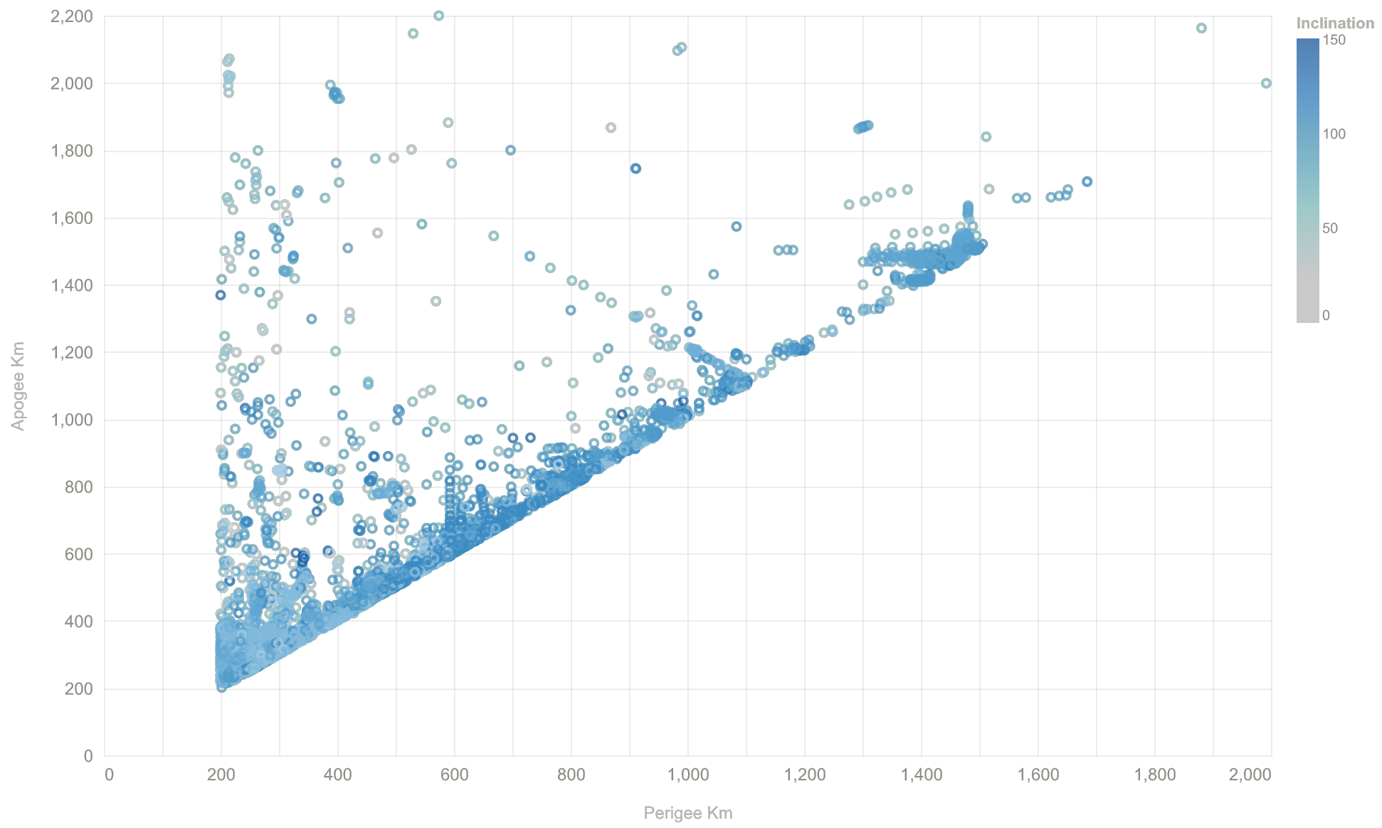
The dataset also has satellite info. Here we plot perigee (lowest point) and apogee (highest point) to understand the structure of our man-made orbiters.
This view zooms into the crowded LEO and low-MEO band, colored by orbital inclination. The lower diagonal edge is circular orbits, where apogee ~ perigee. The dense smear around 530-560 km is the mega-constellation shell - Starlink and friends. The steep run of dark points near the top is the sun-synchronous band, satellites deliberately parked at ~98 degrees so they cross every spot on Earth at the same local time.
Orbit Scatter Query
import satellite;

where
    base_category = 'P'
    and apogee is not null and perigee is not null
    and apogee <= 2200 and perigee >= 200
    and apogee >= perigee - 50
    and inc is not null
select
    perigee as perigee_km,
    apogee::int as apogee_km,
    inc::int as inclination
limit 30000;
The payload explosion
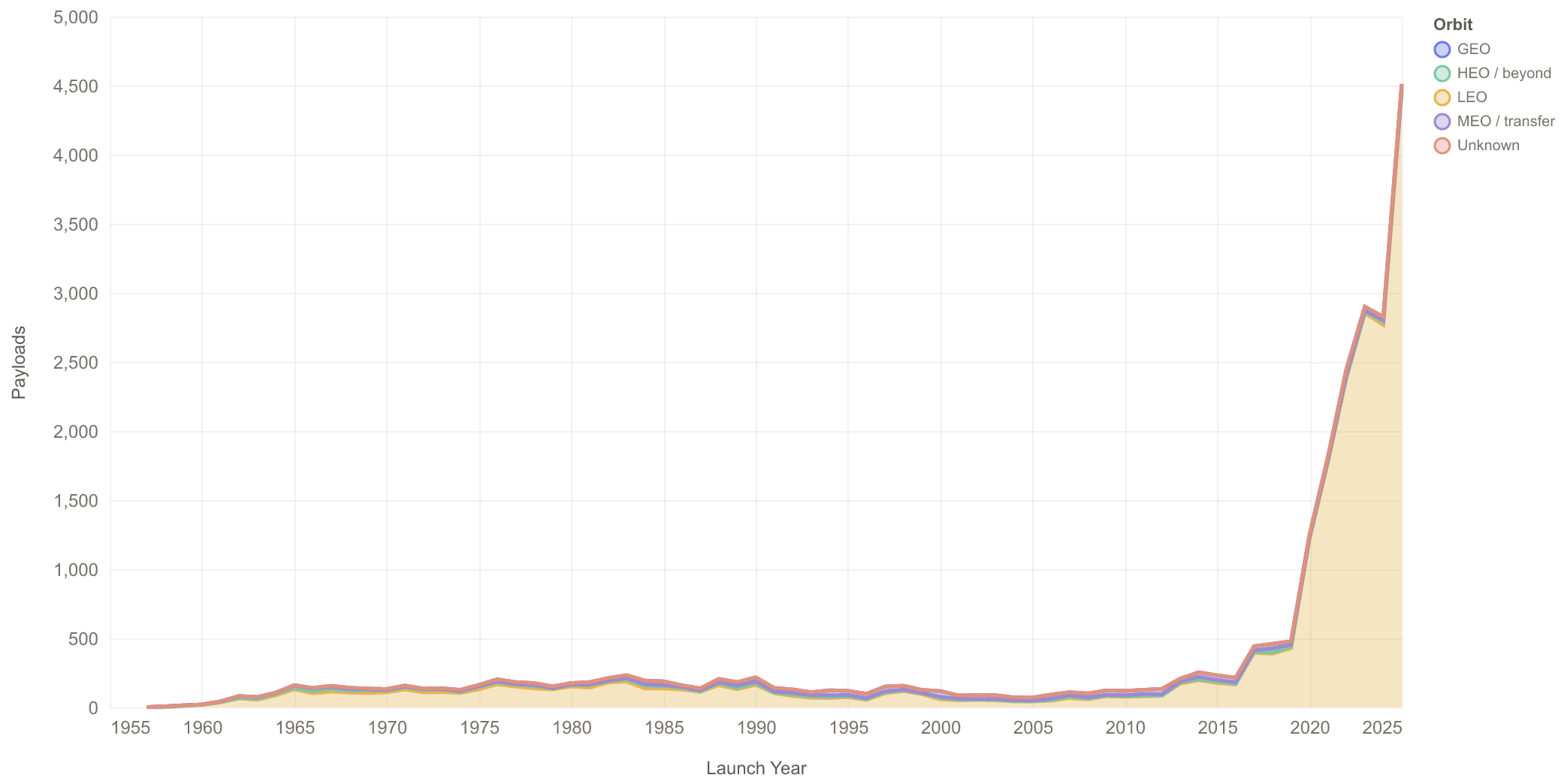
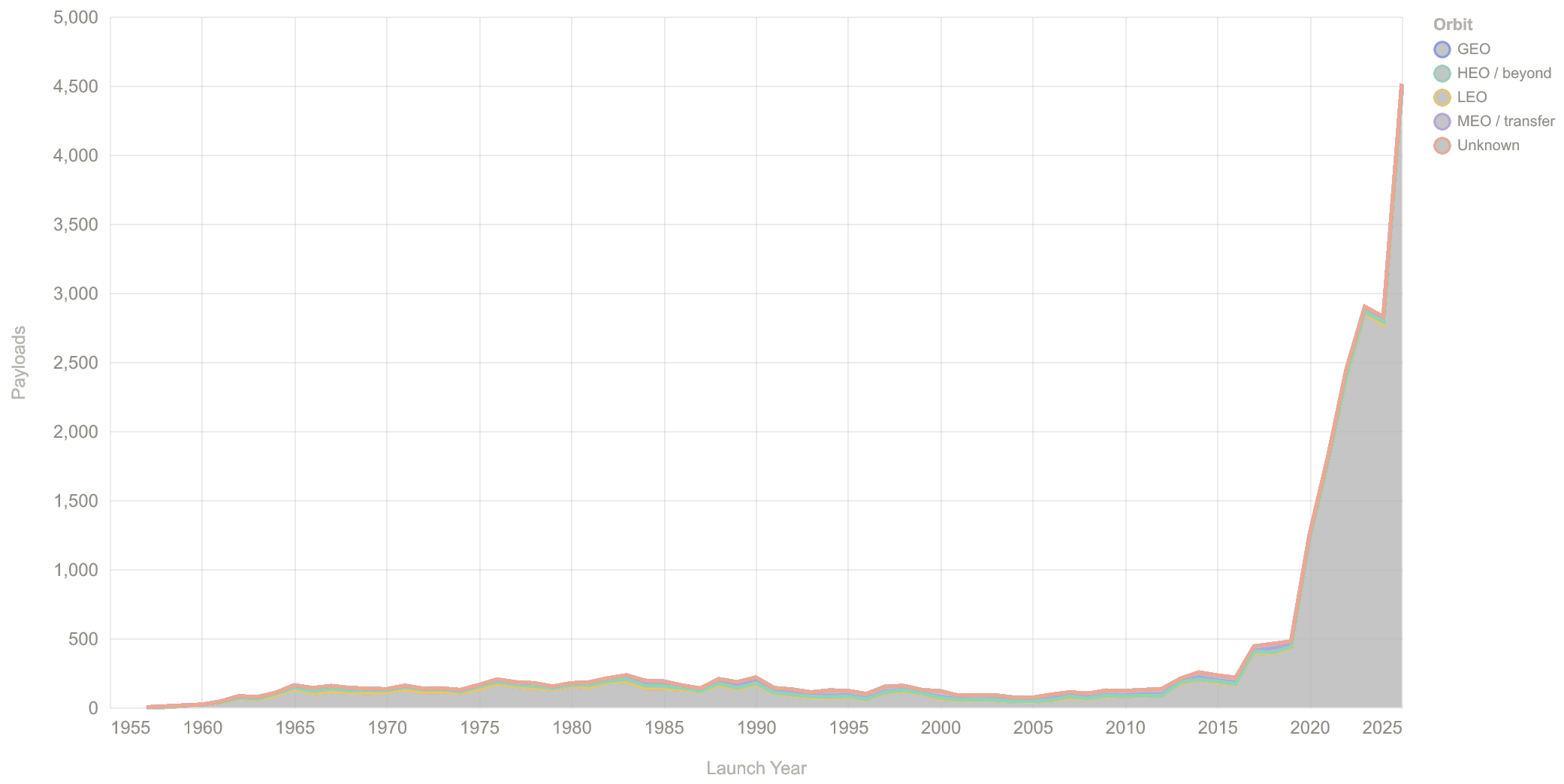
The Cambrian equivalent for rockets is happening now. For sixty years the number of payloads reaching orbit hovered around 100 a year, tracking the launch count above. Then rideshare and mega-constellations decoupled the two: 325 launches carried over 4,500 payloads in 2025. The rocket count grew sharply; the payload count went exponential.
The entire surge is that onegold LEO band - Starlink, PlanetLab, etc stacking thousands of satellites into low orbit where megaconstellations pay covrage dividends.
GEO, MEO, and the deep-space orbits carry on at their decades-old pace, flat along the bottom.
Payloads Per Year Query
import satellite;

where
    base_category = 'P'
    and launch_date.year >= 1957
    and launch_date.year <= 2025
select
    launch_date.year as launch_year,
    CASE
        WHEN apogee is null THEN 'Unknown'
        WHEN apogee <= 2000 THEN 'LEO'
        WHEN apogee <= 34000 THEN 'MEO / transfer'
        WHEN apogee <= 37000 THEN 'GEO'
        ELSE 'HEO / beyond'
    END as orbit,
    count(jcat) as payloads
order by
    launch_year asc;
How the data gets built
The data is hosted on the source website as a bunch of CSV files. We need to do some preprocessing to expose these as tables, and then be able to quickly iterate and extend SQL queries to create our output datasets.
DuckDB can read csv, but these files can have enough warts that it's not super resilient or safe - it's a lot easier to manage the processing in python.
How can we do this?
We'll use the duckdb shell extension to expose python scripts written in uv style directly to duckdb, following this model.
Tips
uv is a fast Python package manager. uv scripts embed their dependencies directly in the file header, making them self-contained and reproducible without a separate requirements.txt.
An example script to ingest satellite data looks like this - we've delegated most of the work on processing the CSV into the arrow format we want to a shared helper. The .tsv is actually the full remote path on the server.
#!/usr/bin/env -S uv run
# /// script
# requires-python = ">=3.13"
# dependencies = ["pyarrow", "requests"]
# ///

from ingest_core import emit, ingest_gcat_file

if __name__ == "__main__":
    table = ingest_gcat_file("tsv/cat/satcat.tsv")
    emit(table)
Once we have that defined, we can define a trilogy datasource that will call that script when it needs to be resolved in a DuckDB query.
root datasource satcat_raw (
    JCAT: jcat,
    Satcat: satcat,
    Launch_Tag: launch.launch_tag,
    Piece: piece,
    Type: type,
    #...lots more fields...
    data_update_date: data_updated_through
    )
grain (jcat)
file `ingest_satcat.py`
freshness by data_updated_through;
One key callout there is the 'freshness by'. In our extraction logic we actually parse out the 'last updated through' text on the gcat homepage, and turn that into a date that is put onto the table.
Since this can be expensive in wall clock time, we don't want to hit the website every time. So we'll define some downstream sources that materialize the same fields to a parquet file in Google Cloud Storage (GCS) which we'll use for default access.
Using this, we can hook up all these sources to a generic trilogy 'refresh' command. When we run this, we'll check the root sources - hitting the website - and then the timestamps from our parquet files; if any are stale, we'll update them.
trilogy refresh data
Then we'll wire up a conditional output dump to JSON for when we do refresh, and use that JSON to serve our website!
Our daily updates then look like this - we can go ahead and schedule that in github actions, and we have an auto-updating website!
 Executing directory: data | Dialect: duck_db | Debug: disabled | Config: data/trilogy.toml

Starting parallel execution:
  Files: 15
  Dependencies: 22
  Max parallelism: 4
  Strategy: eager_bfs
  ✓ etl.preql (1.31s)
  ✓ sites.preql (6.64s) [1 datasource updated]
  ✓ engine.preql (6.70s) [1 datasource updated]
  ✓ platform.preql (6.78s) [1 datasource updated]
  ✓ organization.preql (6.96s) [1 datasource updated]
  ✓ stage.preql (4.17s) [1 datasource updated]
  ✓ vehicle.preql (7.23s) [2 datasources updated]
  ✓ launch.preql (13.62s) [1 datasource updated]
  ✓ core_local.preql (11.40s)
  ✓ debug.preql (11.58s)
  ✓ core.preql (11.75s)
  ✓ satellite.preql (19.20s) [1 datasource updated]
  ✓ satellite_data.preql (16.09s)
  ✓ satellite_data_local.preql (16.32s)
  ✓ debug_satellite.preql (16.74s)
Execution Summary:
  Total Scripts: 15
  Successful: 8
  Noop: 7
  Failed: 0
  Total Duration: 69.41s
  Datasources Updated: 9
Dynamic exploration
The static views above are pre-baked: the refresh job dumps JSON to GCS, and the site renders it on a globe. That's great for the curated story, but the fun part is letting people ask their own questions. We can power a fully dynamic mode that runs entirely in the browser with the same model.
- The daily refresh runs the model against DuckDB on a github actions runner, writing parquet to GCS.
- The charts in this post are generated by DuckDB on a laptop.
- The website's explore mode runs it against DuckDB-WASM, compiled to WebAssembly, running in Chrome/Firefox/Safari.
DuckDB-WASM can read these parquet files over HTTP with range requests - so the browser pulls only the columns and row groups a query touches, no backend required. The semantic model is bundled into the page at build time:
// every data/raw/*.preql file, inlined into the bundle as a string
const preqlModules = import.meta.glob('../../data/raw/*.preql', {
  query: '?raw', import: 'default', eager: true,
})
On top of that sits a chat page. You bring your own API key (or use a limited demo provider), and the model gets handed the Trilogy semantic layer as a tool. When you ask "what rockets have the most engines?" or "plot the top launch sites in Asia," the LLM writes Trilogy, not raw SQL - it works against the tidy concepts (vehicle.stage.engine_count, site.state.e_name) instead of the raw catalog's quirks, and the query executes locally in DuckDB-WASM. The result comes back as a table or a chart you can keep poking at.
This is the payoff of putting the semantic layer at the center. Write the model once, and the same definitions drive a scheduled ETL, a set of hand-built dashboards, a folder of CLI-rendered blog charts, and a natural-language explorer - all just a different engine pointed at the same concepts. (and you can easily swap to a different DB too)
Want to try it yourself? Point your own agent at the gcat_space public model with the Trilogy CLI and every chart in this post is reproducible locally, or open the chat page and start asking.